In this post I plan to show the effects of polyBLEPS and implement a short example program that uses this method to generate bandlimited waveforms, in the hopes of reducing aliasing. In addition, there is also a short overview of some other available methods.

This post was written in the Jupyter Notebook. Notebook is available as .html or as [.ipnyb](Generating Bandlimited Waveforms.ipynb).

Intro

In subtractive synthesis we want to start from waveforms which have a lot of "harmonic content", which we then can "sculpt away" using filters and effects. This usually means sawtooth-waves or square-waves.

In contrast, a sine-wave has very little "harmonic content". In fact, it has the least possible and is so fundamental that it can be seen as the building block of any other signal.

Thus, the square wave can be seen as a summation of certain sin-waves, \begin{equation} f_{\text{square}}(x) = \frac{4}{\pi} \sum_{n=1,3,5,...}^{\infty}{\frac{1}{n} \sin{\left( \frac{n \pi x}{L} \right)}} \, , \label{fourierSeriesSquare} \end{equation}

where $x$, in the context of audio, is our time parameter and $L$ is the square waves period, note that $n$ is defined to be only odd integers (derivation).

Looking at the frequency spectrum of a square wave we can check this...

#Setup
import numpy as np
import scipy
import scipy.signal
import matplotlib.pyplot as plt
import ipywidgets as widgets

L = 1/10;                 # 1 period 0.1s => 10Hz
Fs = 1000                 # samples to take (explained later)
t = np.linspace(0,1,Fs)   # 1sec with 10000 samples
signal = scipy.signal.square(t*(2*np.pi/L)) # 10Hz square wave 

ps = np.abs(np.fft.fft(signal))**2 # power spectrum
freqs = np.fft.fftfreq(signal.size, d=1/Fs) # freqs for plot

#Plot
idx = np.argsort(freqs)
fig, ax = plt.subplots()
ax.xaxis.set_ticks(np.arange(1/L, 100, 1/L))
ax.set_xlim(0,100)
ax.set_title("Frequency spectrum for %d Hz square wave" %(1/L))
ax.set_xlabel("Hz")
ax.plot(freqs[idx], np.sqrt(ps[idx]),".-")

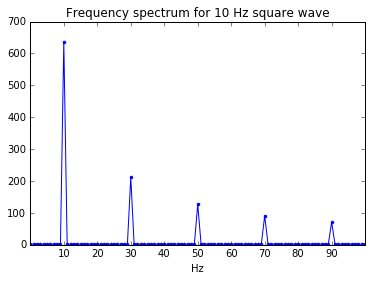
The figure above shows the frequency spectrum of a square wave at 10Hz. From this we can see the individual sin-waves that make up the square wave. The strongest peak is a sin-wave with frequency 10Hz (which usually is referred to as the fundamental). The next peak can be seen at 30Hz, meaning we have a sin-wave at 30Hz but with a lower amplitude. The next peak is at 50Hz, and the next after that at 70Hz, etc. Note that the peaks are missing at even multiples of $\frac{1}{L}$ (20Hz, 40Hz, ...) and have peaks at uneven multiples of $\frac{1}{L}$ (10Hz, 30Hz, ...), just as it was described in \eqref{fourierSeriesSquare}.

In theory these peaks keep showing up all the way up to infinitely high frequencies!

But, when dealing with signals in the digital world, where signals must be sampled at specific time intervals, there is a limit on signal frequencies before we get aliasing.

Aliasing and Nyquist

Aliasing occurs when the signal we are trying to capture has a frequency which is higher than half the sample frequency. When this occurs we can no longer perfectly represent the signal. It has been distorted. The Nyquist theorem says that to perfectly capture a signal through sampling, the sampling frequency must be at least twice that of the highest frequency in the signal.

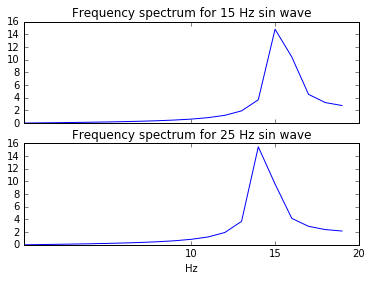
To illustrate aliasing we can look at a sin-wave sampled at 40Hz. A sin-wave with a frequency of 15Hz will have its peak at 15Hz in the frequency spectrum. But a sin-wave at 25Hz is above the threshold of half the sampling frequency and will be aliased. We can see that this means that the frequency of the signal "folds" and appears to go back down in frequency, landing at around 15Hz instead of 25Hz, thus incorrectly representing the signal.

def fft_spectrum(t, signal, Fs):
    """function to help plotting frequency responses"""
    ps = np.abs(np.fft.fft(signal))**2 # power spectrum
    freqs = np.fft.fftfreq(signal.size, d=1/Fs) # freqs for plot
    idx = np.argsort(freqs)
    return (freqs[idx], ps[idx])

def sin_fft(freq, Fs):
    L = 1/freq;               # 1 period 0.1s => 10Hz
    Fs = Fs                   # # of samples to take
    t = np.linspace(0,1,Fs)   # 1sec with Fs samples
    signal = np.sin(t*(2*np.pi/L)) # 1/L Hz sin-wave
    return fft_spectrum(t, signal, Fs)

    #Plot!
    plt.subplots
    fig, ax = plt.subplots(2, sharex=True)
    ax[0].xaxis.set_ticks(np.arange(10, 100, 5))
    ax[0].set_xlim(0,20)
    ax[1].set_xlabel("Hz")

    #15 Hz
    freqs, ps = sin_fft(15, 40)
    ax[0].plot(freqs, np.sqrt(ps))
    ax[0].set_title("Frequency spectrum for %d Hz square wave" %(15))
    #25 Hz
    freqs, ps = sin_fft(25, 40)
    ax[1].plot(freqs, np.sqrt(ps))
    ax[1].set_title("Frequency spectrum for %d Hz square wave" %(25))

From this we can imagine that trying to represent a square wave, which has peaks at infinitely high frequencies can become a bit of a challenge. But why was there no aliasing in the original square-wave example? In that case our sample rate was set to be quite high compared to the period of the square wave. The peaks for the higher frequencies are so small that the effect of aliasing is pretty much negligible.

But if we want to allow square-waves with shorter periods (resulting in a higher fundamental frequency), this can be a problem and introduce unwanted content and noise to our digital signal that arises because of aliasing.

For audio purposes the sampling rate of 44.1kHz is often used. This means that we can represent audio with frequencies up to 20kHz, that is more than what the human ear can pick up. But with aliasing there is risk that higher frequencies than 20k kHz "fold" back and introduce new unwanted frequencies in the audible range.

Methods for Generating Bandlimited Waveforms

How can aliasing be avoided? The signal needs to be Bandlimited. This means that the signal to be represented needs to have no frequency content higher than half the sample rate (or at least that such content has low amplitude).

When recording audio of the real world through a microphone it will almost certainly encounter frequencies which are higher than the sample rate. To avoid aliasing, a lowpass filter is used to make sure that the higher frequencies are sufficiently low, making the signal band limited and thus avoiding aliasing.

When digitally generating waveforms we need to make sure this is also the case. Limit the higher frequencies that can not be sampled. There are multiple methods which can help prevent waveforms from being aliased. Common methods include

• Oversampling
• Additive synthesis
• Band-Limited Step (BLEP)
• Band-Limited Impulse Trains (BLIT)
• Band-Limited rAMP (BLAMP)

The 3 techniques are called quasi-bandlimited, since they do not eliminated aliasing perfectly. They do however, still help reduce the aliasing effects significantly.

Below is a quick overview of the oversampling, additive synthesis techniques and BLEP techniques. The BLEP technique was the one of greatest interest for my project and seemed to fit my needs the best.

I did not get a chance to dive into the other techniques very much. Here are some pointers for for more info on the other ones BLITS and BLAMPS:

BLIT: https://ccrma.stanford.edu/~stilti/papers/blit.pdf

BLAMP: http://www.eurasip.org/Proceedings/Eusipco/Eusipco2016/papers/1570256244.pdf

Oversampling

Here the signal is simply sampled at a high enough frequency that no aliasing occurs or that the effects of aliasing are negligible. Audio is generally sampled at 44.1kHz and if we wish to capture a signal that has high constituent frequencies we must make sure that the sample rate is twice the frequency of the highest constituent frequency. But this can mean that a lot more work has to be done by the computer and might be a problem, especially for realtime applications.

Additive synthesis

Using the fourier series expression for a square-wave above (equation \eqref{fourierSeriesSquare}) we can generate each sample of the signal by manually performing the summation of the constituent frequencies and simply stopping when arriving at the Nyquist frequency. This will get us as close as possible to representing a square-wave without having wrong sounding frequencies caused by aliasing.

def additive_square(N, freq=10, Fs=1000):
    L = 1/freq;               # period
    Fs = Fs                   # # of samples to take
    t = np.linspace(0,1,Fs)   # 1sec with Fs samples
    signal = np.array([0] * len(t), float)
    for i in range(1, len(t)):
        t0 = t[i]
        for n in range(1, N+1):
            signal[i] += 4/np.pi * \
            1/(2*n-1)*np.sin(2*(2*n-1)*np.pi*t0/L)
    return (t, signal)

def plot_additive_square(N, freq, Fs):
    L = 1/freq; 
    print("Highest constituent frequency: %g Hz" \
          % (((2*N-1)*np.pi/L)/(np.pi)) )
    t, signal = additive_square(N, freq, Fs)
    plt.figure(figsize=(14,3))
    plt.subplot(1,2,1)
    plt.plot(t, signal, ".-")
    plt.title("Additive square-wave at %d Hz\n \
    with %d terms, sampled at %d Hz" % (freq, N, Fs))
    plt.xlabel("time [s]")
    
    freqs, ps = fft_spectrum(t, signal, Fs)
    plt.subplot(1,2,2)
    plt.plot(freqs, np.sqrt(ps))
    plt.title("Frequency spectrum of square-wave at %d Hz\n \
    with %d terms, sampled at %d Hz" % (freq, N, Fs))
    plt.xlabel("frequency [Hz]")
    plt.xlim(0,120)

widgets.interact(plot_additive_square, \
                 N=widgets.IntSlider(min=1,max=7,step=1,value=3),\
                 freq=widgets.fixed(18),Fs=widgets.fixed(200))

> Highest constituent frequency: 90 Hz

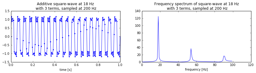
In the figure above we can see an additive square-wave with different values for N sampled at 200Hz. We also the frequency spectrum for this wave. Peaks show up at even intervals as we increase N. But as soon as we hit half of the sampling frequency (100Hz) irregular peaks start to show up, which would cause a non harmonic sound (Not so good for making music). So we can simply stop at the value for N right before crossing the Nyquist frequency, in this case $N = 3$.

When sampling at 44.1kHz and we want to generate a square wave with a fundamental at 420kHz N in this case would be $N = 53$. Depending on the circumstance this might be too many iterations to perform for each sample in a realtime application.

A common approach is to use additive synthesis to generate the wanted waveforms beforehand for different frequencies and store the resulting samples in a wavetable which can then be looked up during runtime. But this requires precomputation and memory.

The Blog-post series at www.earlevel.com provides more information on this.

Band-Limited stEP (BLEP)

This method uses the fact that the step from the low value of the square wave and the high value of the square wave is theoretically instantaneous. So no matter what period or frequency the main square-wave is set to, the part of the wave that does the jump will be always be the same. In digital situation this means that this step can only be as sharp and have as many frequencies as the sample rate allows.

The trick is to have a version of this step that is bandlimited. This "BLEP" can then be substituted in into areas of a naively generated waveform (not taking aliasing into account) that have too steep of a step, thus avoiding the higher frequencies. Since the BLEP will need to be centered around the discontinuity we will need to be able to predict ahead for a few samples when the step will occur, or simply delaying the signal a bit.

These steps can be generated using additive synthesis, described above or by simulating the effect on an impulse being sent through a lowpass filter.

polyBLEP!

(Valimaki and Huovilainen, IEEE SPM, Vol.24, No.2, p.121)

A development on the BLEP method is the so called polyBLEP. Here a polynomial approximation is given for the band limited step function. This allows for quick calculation of the band limited step and does not require memory lookups.

This approximation is arrived at by mathematically interpreting the process of putting a step function through a lowpass-filter. Valimaki and Huovilainen describe the process in their paper. The triangular wave can be used as a function for lowpass filtering, this because its frequency response has the shape of sinc^2. The triangular wave function is given by,

$$ S_{tri}(t) = \begin{cases} t+1 \newline 1-t \newline 0 \end{cases} $$

The frequency response of the triangular pulse can be applied to alter a square wave using convolution. The square wave is convolved with the triangular pulse. During this process the triangular pulse gets integrated.

$$ S_{tri,int}(t) = \begin{cases} 0 \newline \frac{t^2}{2} + t + \frac{1}{2} \newline t - \frac{t^2}{2} + \frac{1}{2} \newline 1 \end{cases} $$

The constant $\frac{1}{2}$-terms are there to ensure continuity. This is the polynomial Band-Limited stEP. The actual correction that is to be applied to a naively generated waveform is given by the BLEP residual. That is, the input impulse subtracted from the BLEP. We get

$$ f_{polyBLEP}(t) = \begin{cases} \frac{t^2}{2} + t + \frac{1}{2} \, , \text{when} \, -1 \leq t \leq 0 \newline t - \frac{t^2}{2} + \frac{1}{2} \, , \text{when} \, 0 \lt t \leq 1 \end{cases} \, . $$

Implementing this in a program means we need some logic to find the discontinuities and then apply the correction. We will need to know in advance when our discontinuities show up in order to apply the correction, but since the waveforms are periodic this should not be too difficult.

Below is an example of generating a square wave corrected with the help of polyBLEPS.

# PolyBLEP by Tale
# http://www.kvraudio.com/forum/viewtopic.php?t=375517
# (adapted a bit by me)

#double t = 0.; // 0 <= t < 1
#double dt = freq / sample_rate;
def poly_blep(t, dt):
    """gives the polyblep correction for a 
    discontinuity given in a naively generated waveform.
    dt = freq/Fs
    """
    if (t < dt):              # 0 <= t < 1
        t /= dt;
        # 2 * (t - t^2/2 - 0.5)
        return t+t - t*t - 1
    elif (t > 1. - dt):       # -1 < t < 0
        t = (t - 1.) / dt;
        # 2 * (t^2/2 + t + 0.5)
        return t*t + t+t + 1
    else:                     # 0 otherwise
        return 0

def poly_square(t, dt, aa):
    naive_square = 0
    if t <= 0.5:
        naive_square = 1;
    if t > 0.5:
        naive_square = -1;
    if aa:
        #with polyBlep correction.
        #one for the raise and one for the fall (at 0.5)
        return naive_square + poly_blep(t, dt) \
                            - poly_blep((t+0.5) % 1, dt)
    else:
        return naive_square
    
t = 0
Fs = 3520
f0 = 240
dt = f0/Fs

out_no_aa = np.array([0]*Fs, float)
out_aa = np.array([0]*Fs, float)

# make sawtooth wave f0 times
t = np.linspace(0,f0,Fs)

for i in range(0,len(t)):
    t_tmp = t[i] % 1
    out_no_aa[i] = poly_square(t_tmp, dt, 0)
    out_aa[i] = poly_square(t_tmp, dt, 1)

t = np.linspace(0,1,Fs) #f0 times in 1 second
signal_no_aa = out_no_aa
signal_aa = out_aa

We can see the effect this has on aliasing by looking at the frequency response.

#Plot!
plt.figure(figsize=(16,20))
plt.subplot(4,2,1)
plt.plot(t, signal_aa, ".-")
plt.title("Square with polyBLEP")
plt.xlabel("time [s]")
plt.xlim(0,0.05); plt.ylim(-2,2)
plt.subplot(4,2,2)
plt.plot(t, signal_no_aa, ".-")
plt.title("Square without polyBLEP")
plt.xlabel("time [s]")
plt.xlim(0,0.05); plt.ylim(-2,2)

freqs, ps = fft_spectrum(t, signal_aa, Fs)
plt.subplot(4,2,3)
plt.plot(freqs, np.sqrt(ps),".-")
plt.title("Frequency response with polyBLEP")
plt.xlabel("frequency [Hz]")
plt.xlim(0,2000)
plt.ylim(0,400)

freqs, ps = fft_spectrum(t, signal_no_aa, Fs)
plt.subplot(4,2,4)
plt.plot(freqs, np.sqrt(ps),".-")
plt.title("Frequency response without polyBLEP")
plt.xlabel("frequency [Hz]")
plt.xlim(0,2000)
plt.ylim(0,400)

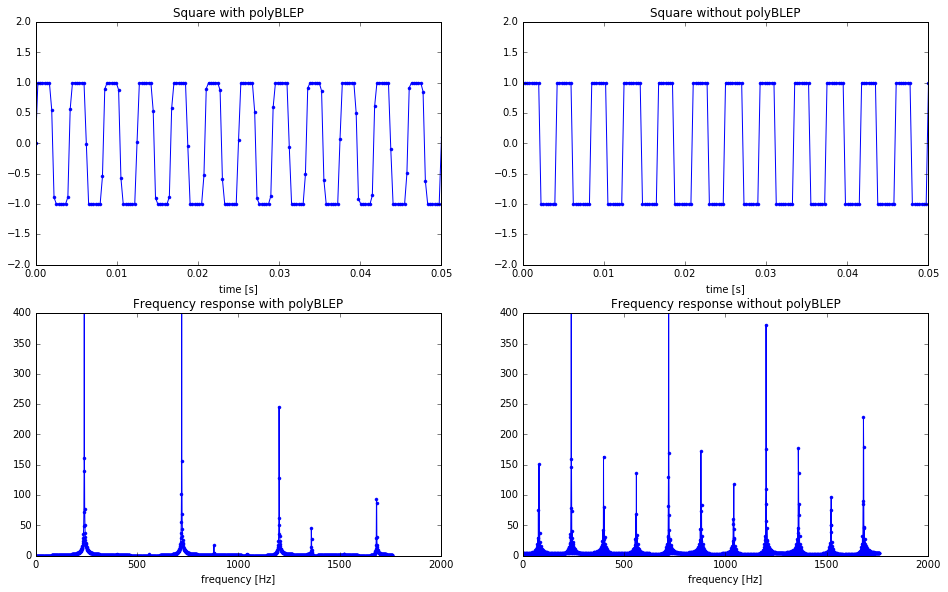
There we have it. In the signal without polyBLEPS we see a lot of unwanted frequencies. Any peaks with a height around 150 or below could be considered aliasing (except for maybe at the last peak). When adjusting the signal using the polyBLEP correction we se a dramatic reduction in aliasing!

Below are two videos where you can hear the effects of the polyBLEPS. Here a sample rate of 22050 was used. VOLUME WARNING!

Without polyBLEP:

With polyBLEP:

A pretty dramatic effect that makes the generated sounds much cleaner, especially for higher notes!